1. The basic principle
1.1. A look back into the past
Because Checkmk continuously monitors all hosts and services at regular intervals, it provides an exceptional basis for the later evaluation of their availability. And not only that — it can also be calculated for what percentage of a given time range an object was in a specified state or states, how often this state occurred, the duration of its longest stop, and much more.
Every calculation is based on a selection of objects and a specified time range in the past. Checkmk then reconstructs, within this time range, a chronological sequence of the states of all of the selected objects. Per state the times will be added together and displayed in a table. This table can, for example, show that a particular service experienced states of 99.95 % OK, and 0.005 % WARN over the defined time range.
When making such calculations, Checkmk also correctly takes account of such factors as scheduled downtimes, service downtimes, unmonitored time ranges and other special factors, enables the summary of states, and the ignoring of ‘brief interruptions’. Numerous customization options are also available. An availability of BI aggregations is also possible.
1.2. Possible states
Through the inclusion of scheduled downtimes and similar special states, there is in theory a large number of possible combinations of states, for example: CRIT + In Planned Downtime + In Service Time + Flapping. Because most such combinations are not very useful, Checkmk reduces these to a small number and in doing so proceeds according to a principle of priorities. Since in the above example the service was in a scheduled downtime, the state in scheduled downtime simply applies, and the actual state is ignored. This reduces the list of possible states to the following:
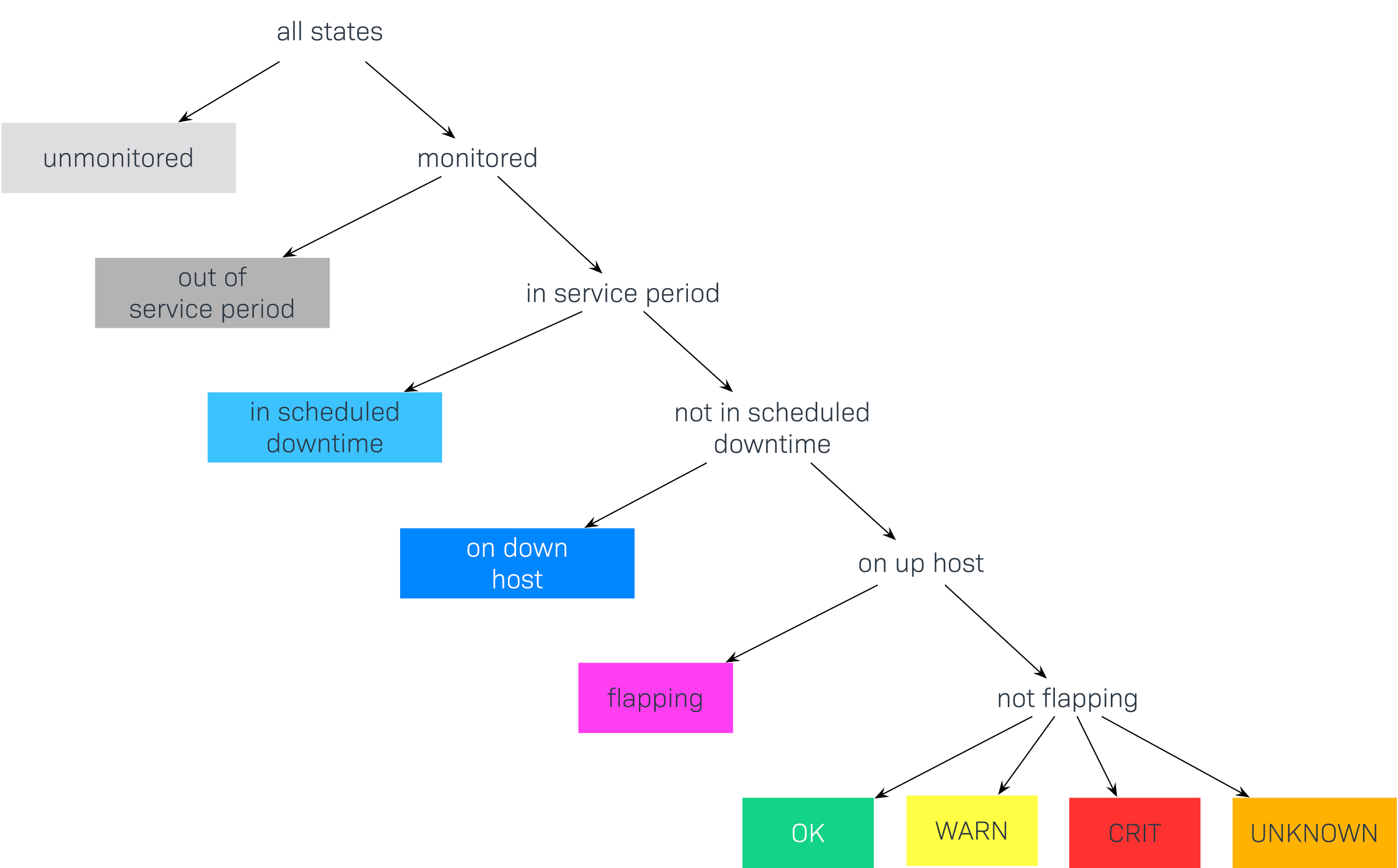
This graphic shows the order in which states are prioritized. Later we will show how some states can be ignored or combined. Here are the states again, in detail:
| State | Abbreviation | Description |
|---|---|---|
unmonitored |
N/A |
Time ranges during which the object was not being monitored. There are two possible reasons for this: the object was not in the monitoring’s configuration, or the monitoring itself was not running during the specified time range. |
out of service period |
The object was outside its service period |
|
in scheduled downtime |
Downtime |
The object was in a period of scheduled downtime |
on down host |
H.Down |
This state is only available for services — when the service’s host is (down). A monitoring of the service at this time is not possible. For most services this has the same meaning as if the service is CRIT — but not for all! For example, the state of a (File system-Check) is certainly independent of the host’s accessibility. |
flapping |
Phases in which the state is |
|
UP DOWN UNREACH |
Monitoring states for hosts |
|
OK WARN CRIT UNKNOWN |
Monitoring states for services and BI aggregations |
2. Availability retrieval
2.1. From the view to the analysis
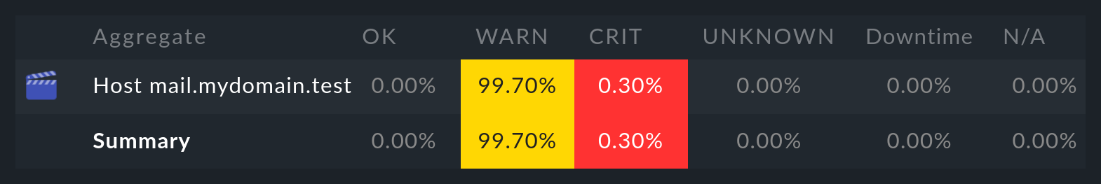
Generating an availability analysis is very simple. First retrieve any view of hosts, services or BI aggregations. There you will find in the menu Services menu the Availability item, which takes you directly to the calculation of the availability of the selected objects. The data will be displayed as a table:
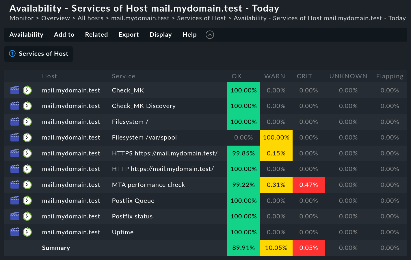
The table shows the same objects that were seen in the preceding view. Shown in each column is the proportion of the requested time range an object was in the state being queried. The value is given as a percentage, by default to two decimal places — which you can also easily customize.
The time range query can be customized with the Availability > Change display options > Time Range menu item. More on this later…
You have the option of receiving the table as a PDF (commercial editions only). A download of the data in the CSV-Format is also possible (Export as CSV). It will look like this for the above example:
Host;Service;OK;WARN;CRIT;UNKNOWN;Flapping;H.Down;Downtime;N/A
mail.mydomain.test;Check_MK;100.00%;0.00%;0.00%;0.00%;0.00%;0.00%;0.00%;0.00%
mail.mydomain.test;Check_MK Discovery;100.00%;0.00%;0.00%;0.00%;0.00%;0.00%;0.00%;0.00%
mail.mydomain.test;Filesystem /;100.00%;0.00%;0.00%;0.00%;0.00%;0.00%;0.00%;0.00%
mail.mydomain.test;Filesystem /var/spool;0.00%;100.00%;0.00%;0.00%;0.00%;0.00%;0.00%;0.00%
mail.mydomain.test;HTTP https://mail.mydomain.test/;99.85%;0.15%;0.00%;0.00%;0.00%;0.00%;0.00%;0.00%
mail.mydomain.test;HTTPS https://mail.mydomain.test/;100.00%;0.00%;0.00%;0.00%;0.00%;0.00%;0.00%;0.00%
mail.mydomain.test;MTA performance check;99.23%;0.30%;0.46%;0.00%;0.00%;0.00%;0.00%;0.00%
mail.mydomain.test;Postfix Queue;100.00%;0.00%;0.00%;0.00%;0.00%;0.00%;0.00%;0.00%
mail.mydomain.test;Postfix status;100.00%;0.00%;0.00%;0.00%;0.00%;0.00%;0.00%;0.00%
mail.mydomain.test;Uptime;100.00%;0.00%;0.00%;0.00%;0.00%;0.00%;0.00%;0.00%
Summary;;89.91%;10.05%;0.05%;0.00%;0.00%;0.00%;0.00%;0.00%
With the help of an automation user, which can
authenticate itself via the URL, you can also retrieve data — e.g., with
wget or curl) — and automatically process the data under
script control.
2.2. Timeline display
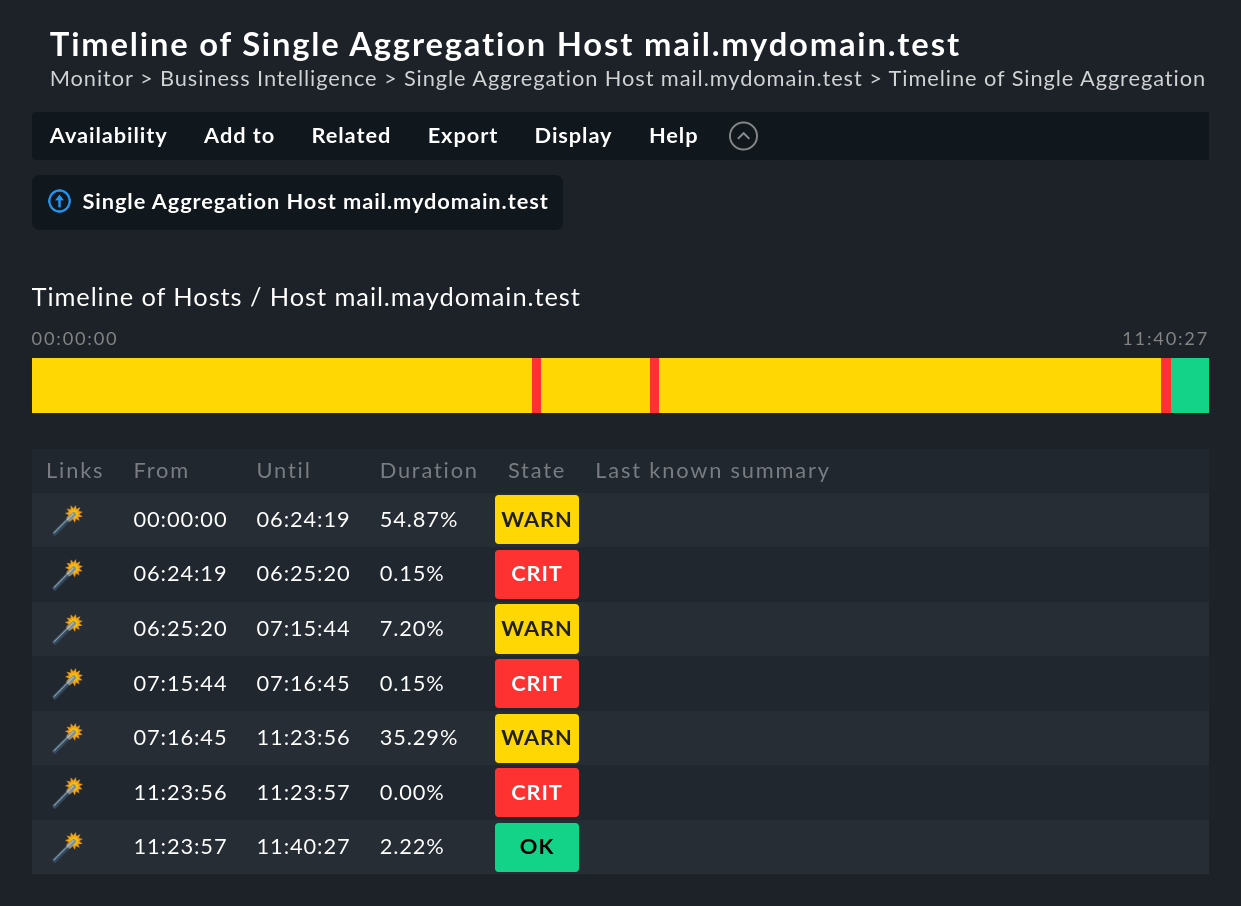
The ![]() symbol can be found in every line of the table.
This button takes you to a timeline display for the relevant object,
in which it is precisely itemized which state change(s) occurred in
the specified time range (abbreviated here):
symbol can be found in every line of the table.
This button takes you to a timeline display for the relevant object,
in which it is precisely itemized which state change(s) occurred in
the specified time range (abbreviated here):
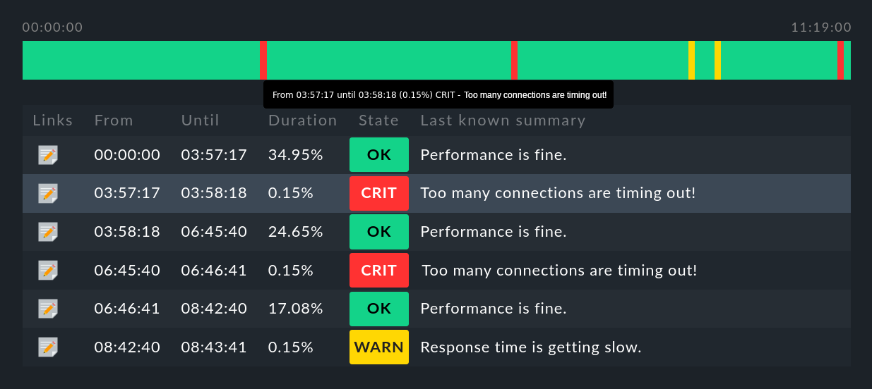
Some useful tips:
Hover the mouse cursor over a timeline symbol in a object’s line in the display, this will be highlighted in the table display.
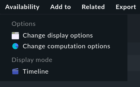
Also in the timeline, you can use the Availability > Change display options or Availability > Change computation options menu items to customize the options for display and evaluation.
With the
 symbol you can add an Annotation to the selected item. Here you can also retrospectively post downtimes (more on this in the next section).
Under the availability of BI aggregations, with the
 magic wand symbol you can time travel to the state of the aggregate for the time slice in question. More on this below.
Using the Availability > Timeline menu item in the main view, you can view the timelines of all selected objects in a long, single page.
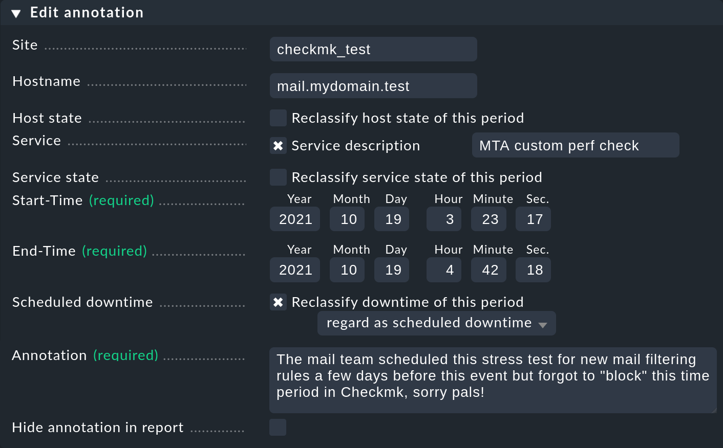
2.3. Annotations and subsequent downtimes
As just mentioned, with the ![]() symbol the timelines
offer the possibility of adding an annotation to a time period.
A pre-filled form (‘Properties’) is provided into which comments can be entered:
symbol the timelines
offer the possibility of adding an annotation to a time period.
A pre-filled form (‘Properties’) is provided into which comments can be entered:
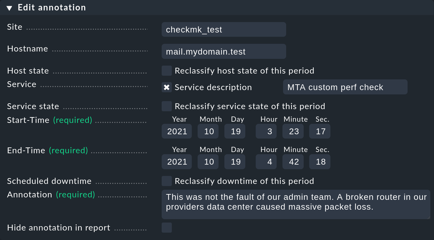
With this you can define and extend the time range with different values as required. This is, for example, practical if you wish to annotate a larger time slice that has experienced repeated state changes. If you omit entering a service, the annotation will be created for the host. This will then be automatically related to all of the host’s services.
In every availability view all annotations applicable to the time range and the objects being displayed will be automatically visible.
But annotations have an additional function. Downtimes can be retrospectively entered — or conversely, removed. The availability analysis takes these corrections into account in exactly the same way as with ‘normal’ downtimes. There are at least two legitimate justifications for this:
During operations it can happen that planned downtimes are incorrectly entered. This of course is bad for the accuracy of the availability statistics. Through retrospective entering of these times the reporting can thus be rectified.
There are users who misuse downtimes during a spontaneous outage in order to suppress a notification. This effectively corrupts the later analysis. This can be corrected retrospectively by deleting the erroneous downtime.
To reclassify downtimes, simply select the Reclassify downtime of this period checkbox:
2.4. Displaying monitoring history
In the availability table, alongside the symbol for the timeline a further
symbol can be found: ![]() . This takes you to a
view of the monitoring history with a pre-filled filter for the relevant
object and the time range for the query. Here you will not only see the event
on which the availability analysis is based (the state changes),
but also the associated notifications and similar events:
. This takes you to a
view of the monitoring history with a pre-filled filter for the relevant
object and the time range for the query. Here you will not only see the event
on which the availability analysis is based (the state changes),
but also the associated notifications and similar events:
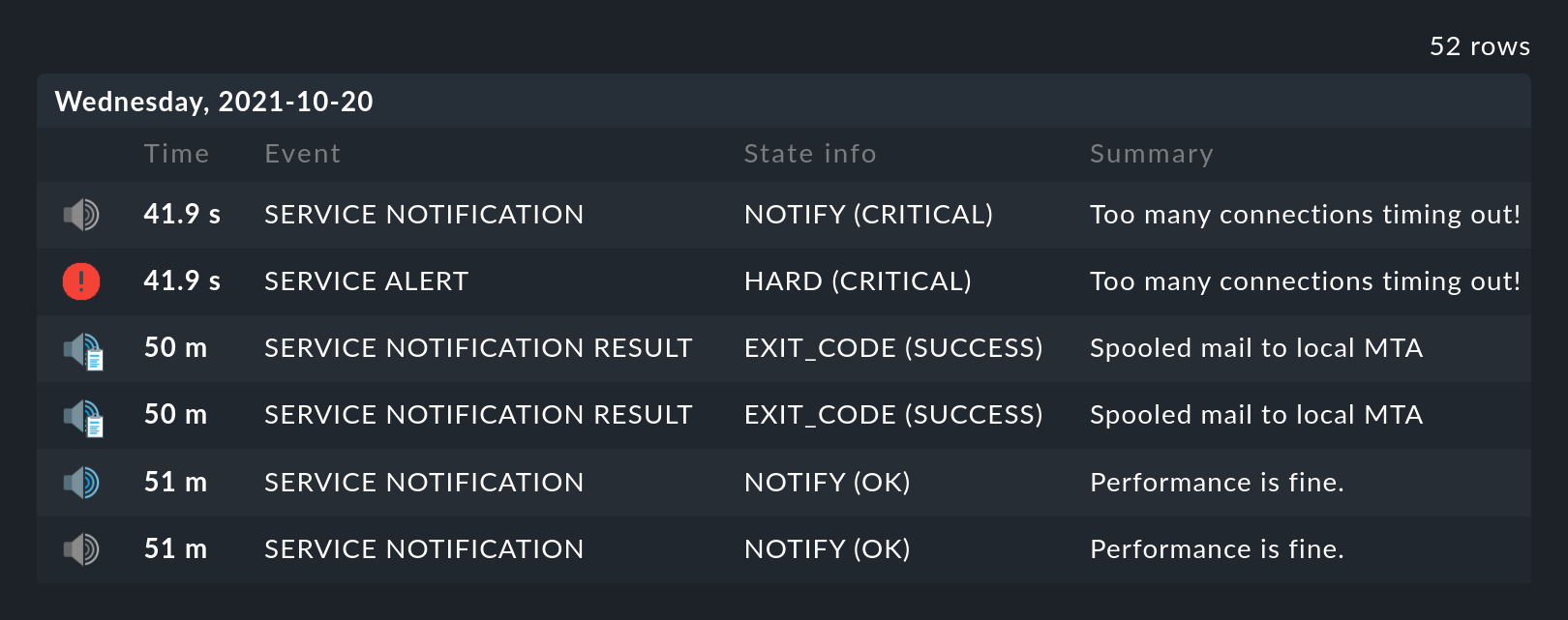
What is not visible here is the state of the object at the start of the query’s time period. The availability calculation looks even further back into the past in order to reliably determine the starting state reliably.
3. Calculation options
As well as the calculation itself, the availability display can also be controlled using numerous options. You can find them in the Availability > Change display options respectively Availability > Change computation options menu items.
Once the options have been altered and confirmed with Apply, the availability will be recalculated and displayed. All of the changed options will be stored in the user’s profile as the default, so that subsequent queries will use the same settings.
At the same time the options will be coded into the current page’s URL. If you now save a Bookmark on the page — e.g., using the practical Bookmarks-element — the options will be a part of this, and when later clicked-on will be generated in exactly the same way.
3.1. Choosing the time range
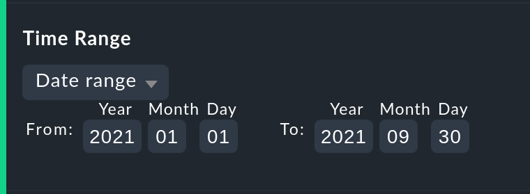
The first and most important option in any availability calculation is of course
the time range to be examined. In Date range a time range with precise start
and end dates can be specified.
The final day — up until 24:00 — will be included.

Much more practical are the relative time specifications, such as, for example, Last week. Exactly which time range will be displayed — intentionally — depends on the point of time at which the calculation is made. Note — here "one week" always refers to a range from Monday 00:00 until Sunday 24:00.
3.2. Options affecting displays
Many options influence the format of the displays, while others in turn influence the calculation methods. To begin with, let’s look at the displays:
Hide lines with 100 % availability
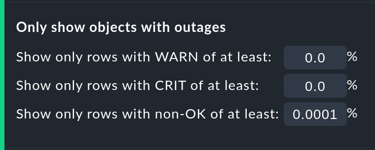
The Only show objects with outages option limits the display to such objects
that really have outages — i.e., times when the state was not OK or UP.
This is useful where there are a large number of services, from which only those
few that actually have problems are of interest.
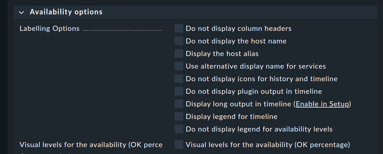
Labelling options
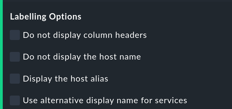
The Labelling options allow various label fields to be activated or deactivated. Some of the options are primarily interesting for Reporting. If, for instance, a report is to be produced for a single host, then the column for the host name is not really required.
The alternative display names for services can be defined using a rule, and by using these, for example, displays for important services can be given a name that is explicit and meaningful for the report’s reader.
Using colors when displaying SLAs with thresholds
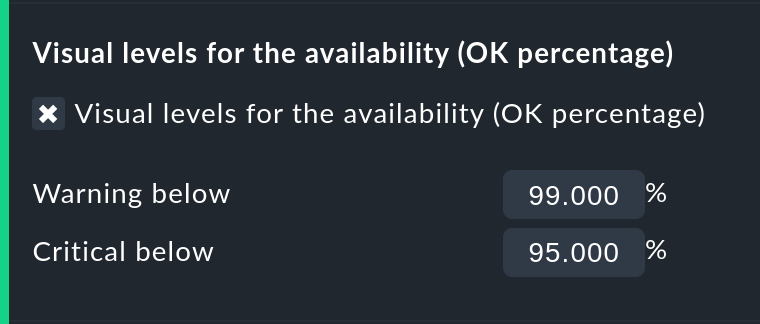
With Visual levels you can highlight objects that have not maintained a specified availability within the queried time range. This applies only to the column for the OK-state. This is normally always green. A shortfall for the defined threshold will cause the color of this cell to change from green to yellow, or to red. This could be described as a very simple SLA-overview.
Displaying the number and duration of the individual outages
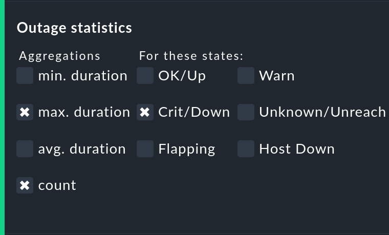
The Outage statistics option provides additional information columns in the availability table. In the screenshot below it can be seen that the additional information for max. duration and count have been activated for the Crit/Down status column. This means that for outages with a CRIT/DOWN state, the number of incidents, as well as the duration of the longest incident respectively, are shown.
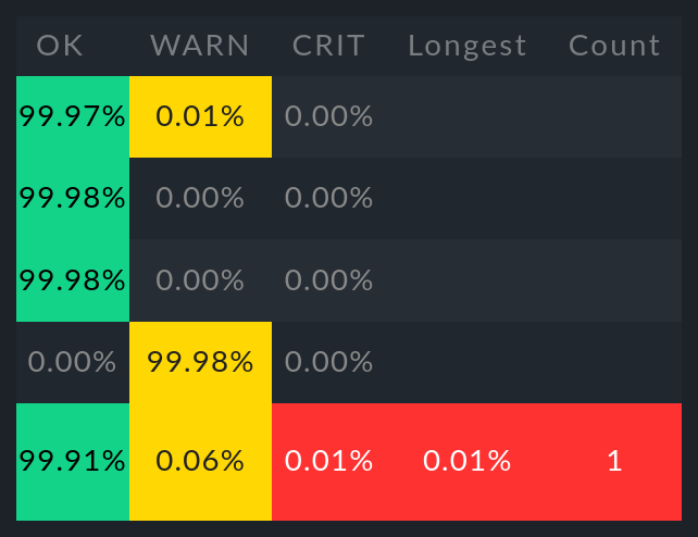
In the table these additional columns will be created.
Time specification display
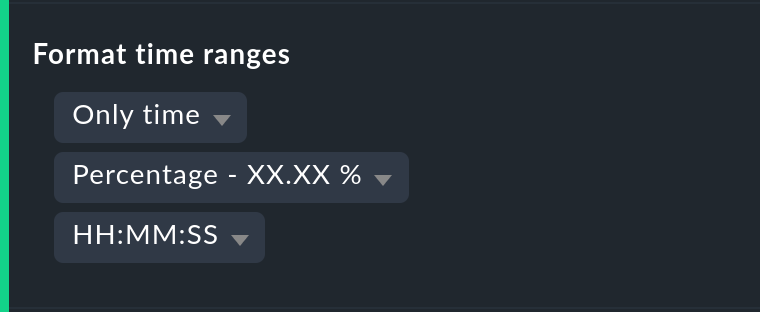
It is not always wise to specify (un)availabilities as percentages. The Format time ranges option enables switching to a display that presents the time ranges as absolute values. With this the total duration of the outages can be seen to the exact minute. The display even shows seconds, but note that that this only makes sense if the monitoring is conducted at one-second intervals, and not as is customary with one check per minute. Likewise the specification’s precision (the number of decimal places in the percentage values) can be defined.

The formatting of time stamps applies to settings in the Timeline. A changeover to UNIX-Epochs (seconds elapsed since 1.1.1970) simplifies the correlation of time ranges to the appropriate locations in the monitoring history’s log data.
Customizing the summary line

Not only can the summary in the table’s last line be activated/deactivated with this — you can also decide between a total sum and an average. For columns containing a percentage value, using the Sum setting will result in an average being shown, since adding percentage values makes little sense.
Showing the small timeline

This option adds a miniature version of the availability timeline directly to the results table. It corresponds to the graphic bar in the detailed timeline, but is smaller and is integrated directly into the table. In addition, it is true to scale, so that multiple objects can be compared in the same table.
Grouping by host, host group or service group

Independently of the display from which you are coming, the availability always shows all objects in a common table. With this option you can select a grouping by host, by host group, or by service group — each group will then get its own Summary-line.
Note that with a grouping by service group, services can appear multiply, since services can be allocated to multiple groups simultaneously.
Only display availability

The Availability option ensures that only the column for the OK or (UP states will be displayed — with the title Avail.. In this way only the actual availability will shown. This option can be combined with the further options explained below, with other states (e.g., WARN), and can also include the OK-state and thus be assessed as available.
3.3. Grouping of states
The states described in the introduction can be customized and condensed in very many ways. In this way very different forms of evaluation can be flexibly generated. The are various options for this.
Handling the WARN, UNKNOWN and Host Down states
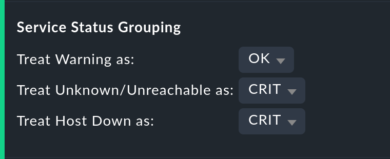
The Service status grouping option provides the possibility of showing various ‘intermediate states’. A common situation is to force WARN to be treated as OK. This can be quite useful if you are interested in a service’s actual availability. Often WARN doesn’t mean a real problem exists yet, but could soon develop. Thus, looked at in this way, WARN must be regarded as available. With network services such as an HTTP-server, it is certainly sensible to treat times during which the host is DOWN in the same manner as when the service is CRIT.
The states that are omitted due to the regrouping will of course also be missing from the results table, which will have fewer columns.

The Host status grouping option is very similar, but it relates to the availability of hosts. The UNREACH state means that a host, due to network problems, cannot be monitored by Checkmk. In such situations, for the purposes of the availability calculations you can decide whether you prefer to treat the UNREACH state as UP or DOWN. The default is to treat UNREACH as its own state.
Handling of unmonitored time periods and flapping
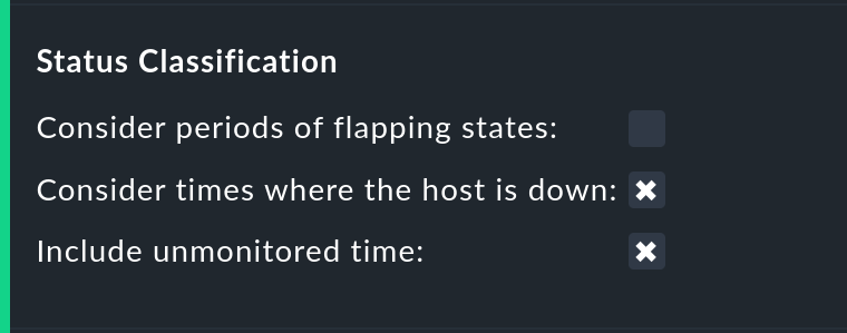
In the Status classification option further summaries will be undertaken.
The Consider periods of flapping states check box is on by
default — with this phases of frequent state changes constitute their own
state: ![]() — ‘flapping’. The idea behind this is
that even though it can be said that at such times the affected service always
returns to the OK state, due to the frequent outages the service is
effectively unusable.
By deactivating this option the concept of ‘flapping’ will then be completely
ignored, and the respective actual state will reappear — and the flapping
column will also be removed from the table.
— ‘flapping’. The idea behind this is
that even though it can be said that at such times the affected service always
returns to the OK state, due to the frequent outages the service is
effectively unusable.
By deactivating this option the concept of ‘flapping’ will then be completely
ignored, and the respective actual state will reappear — and the flapping
column will also be removed from the table.
Removing the Consider times where the host is down option works in a similar way. The concept of Host down is deactivated. This option only makes sense for the availability of services. In phases during which the host is not UP, the actual state of the service will be taken as the basis for the availability — or more precisely, the state of the last Check before the host became unavailable. This can be sensible with services for which their accessibility over the network is not relevant.
The Include unmonitored time option is also similar. Assume that an analysis for February is to be made, and that a particular service has only been in the monitoring since the 15th of February. Does this service then have an availability of only 50 %? With the default setting — option active — this will actually be the case. The missing 50 % will not be assessed as outage, rather it will be added-together in its own column under the title N/A. Without the option it will correspond to 100 % of the time from the 15th to the 28th of February. This does however mean that a one hour outage for this service will be reflected as double the percentage of a service that has been monitored for the whole month.
Handling of scheduled downtimes
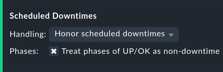
With the Scheduled Downtimes option you can specify how scheduled downtimes affect the availability analysis:
Honor scheduled downtimes is the default. Here downtimes will be treated as their own state and summarized in their own column. With Treat phases of UP/OK as non-downtime you can subtract the times during which, despite the downtime, the service was OK.
Ignore scheduled downtimes is treated as if no downtime had been entered. Outages are outages — full stop. Of course then only if an outage really occurred.
Exclude scheduled downtimes means that the scheduled downtimes are simply excluded from the time period being analyzed. The percentage for the availability then corresponds to the times outside the scheduled downtimes.
Merging equal phases

Through the conversion of one state to another (e.g., from WARN to OK) it can occur that consecutive sections of an object’s timeline will have the same state. Normally such sections will be merged into a single section. This is generally a good thing, and clear, but it does has an effect on the display of the details in the timeline, and possibly also the counting of events with the Outage statistics option. You can therefore deactivate this merging with the Do not merge consecutive phases with equal state option.
3.4. Ignoring short interruptions
Sometimes monitoring often produce momentary problem messages, but under normal conditions the object is already OK by the time the next check runs (after one minute) — and no way has been found through adjusting thresholds or similar to get a neat grip on such cases. A common solution is to set the Maximum number of check attempts from 1 to 3 to allow more failures before a notification is triggered. Thus the concept of Soft states has been developed — meaning the WARN, CRIT or UNKNOWN states — as long as all of the permitted attempts have not been ‘used up’.
We are occasionally asked by users who use this feature why Checkmk’s Availability Module has no function for calculating using only Hard states. The reason for this: There is a better solution! One could use the hard states as the basis…
… so that real outages, due to the unsuccessful first and second check attempts, will be assessed as being two minutes too short.
… and one could not retrospectively readjust the behavior for short outages.

The Short time Intervals option is much more flexible and at the same time very simple. Simply define a length of time which must be exceeded before the states will be evaluated.
Assume that the time value has been set to 2.5 minutes (150 seconds). If a service has been continuously OK, then is CRIT for 2 minutes, and then reverts to OK, the short CRIT-interval will simply be assessed as OK! The opposite situation incidentally also works! A short OK within a long WARN-phase will likewise be assessed as WARN.
Generally speaking, short intervals for which before and after the same state prevails will receive that same state. For a sequence of OK, then a 2 minute WARN, followed by CRIT, the WARN will persist — even if it was of a shorter duration than the defined length of time!
Bear in mind when defining the time, that in Checkmk the standard check interval is one minute. Thus every state has a duration of multiples of approximately one minute. Because the agent’s actual response times vary slightly, this can easily be 61 or 59 seconds. Therefore it is safer to not enter exact minutes for the value, rather to include a buffer — hence the example with 2.5 minutes.
3.5. Effect of time periods
An important function of the availability calculations in Checkmk is that they can be made dependent on time periods. With this times can be defined for every individual host or service. In these times the host/service will be expected to be available and the state then used for the calculations. Therefore every object has the Service period attribute. The procedure is as follows:
Define a time period for the service times.
Assign these to the objects with the Host & Service parameters > Monitoring configuration > Service period for hosts or respectively the … for services rule sets.
Activate the changes.
Use the Service time Availability-option to control the behavior:
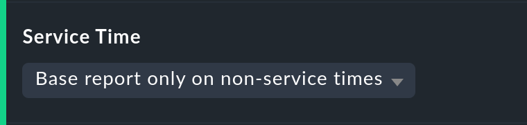
Here there are three simple possibilities. The default Base report only on service times hides times outside the defined service times. These hidden times then don’t count towards the 100 %. Only the time ranges within the service times will be actually considered. In the timeline display the remaining times will be ‘grayed-out’.
Base report only on non-service times performs the opposite, and and in effect calculates the inverse display: How good was the availability outside the service times?
The third option Include both service and non-service times deactivates the complete concept of service times and shows the calculations for all times from Monday 00:00 to Sunday 24:00.
By the way: If a host is not in the service time, for Checkmk it does not automatically mean that this also applies to the services on the host. Services always require their own rule in Service period for services.
The notification period
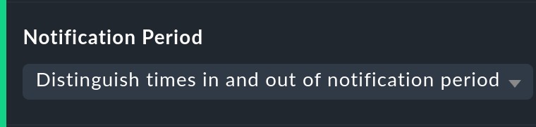
There is incidentally another related option: Notification period. Here the notification period for the evaluation can also be drawn on. This was actually only conceived so that for particular times no notifications for problems would be generated, and does not necessarily cover the service time. This option was introduced in the past when the software did not yet work with a service time, and nowadays it has only been retained for compatibility reasons. It is better not to use it.
3.6. Limiting the calculation time
When calculating availability, the complete history of the selected object must
be reopened. How that works in detail can be learned
further below. Especially in ![]() Checkmk Raw, the analysis
can take some time, since its core has no cache for the required data and the
text-based log data must be sequentially searched.
Checkmk Raw, the analysis
can take some time, since its core has no cache for the required data and the
text-based log data must be sequentially searched.
So that an excessively-complex query — that may possibly have been started unintentionally — does not tie up an Apache process, consume CPU and thus ‘hangs’, there are two options to limit the calculation’s duration. Both are activated by default:
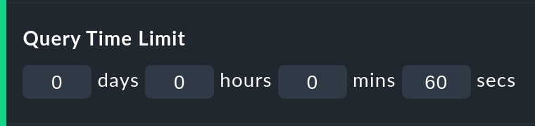
The Query time limit limits the duration of the underlying query to the monitoring core to a specified time. This is predefined as thirty seconds. If this time is exceeded the analysis will be aborted and an error highlighted. If you are certain that the analysis can be allowed to run for longer, simply raise the timeout manually.

The Limit processed data option protects from calculations with many objects. Here a limit will be applied that functions analogous to that in the views. If the query to the monitoring core will produce more than 5000 time periods, the calculation will be aborted with a warning. The limitation will have been pre-processed in the core — where the data is gathered.
4. Availability in Business Intelligence
4.1. The basic principle
A powerful feature of Checkmk’s availability calculation is the facility to calculate the availability from BI aggregations. The big attraction here is that for this purpose Checkmk retroactively reconstructs the precise state of the respective aggregates at a particular point in time by using the protocols of the states of the individual hosts and services.
Why so much time and effort? Why not just query the BI aggregation with an active Check, and then show its availability? Well, the effort has quite a number of advantages for the user:
The construction of BI aggregations can be adapted retrospectively, and then the availability can be recalculated.
The calculation is more precise, since by not using an active check an inaccuracy of +/- one minute is not generated.
An excellent analysis function is available, with which the exact cause of an outage can be retrospectively investigated.
More importantly, an extra check must not be created.
4.2. Availability retrieval
Retrieving the availability view is initially analogous to that for the hosts and services.
Select a view with one or more BI aggregations, and select the BI Aggregations > Availability menu item.
Here there is also a second method — every BI aggregation has a direct path
to its availability using the ![]() symbol:
symbol:
In itself the calculation is initially analogous to that for the services, however without the Host down and flapping columns, since these states do not exist for BI:
4.3. Time travel
The big difference is in the ![]() time line view.
The following example shows an aggregate in our demo server, which was CRIT
for a very brief interval of one second (this would be a good example for the
use of the Short time intervals option).
time line view.
The following example shows an aggregate in our demo server, which was CRIT
for a very brief interval of one second (this would be a good example for the
use of the Short time intervals option).
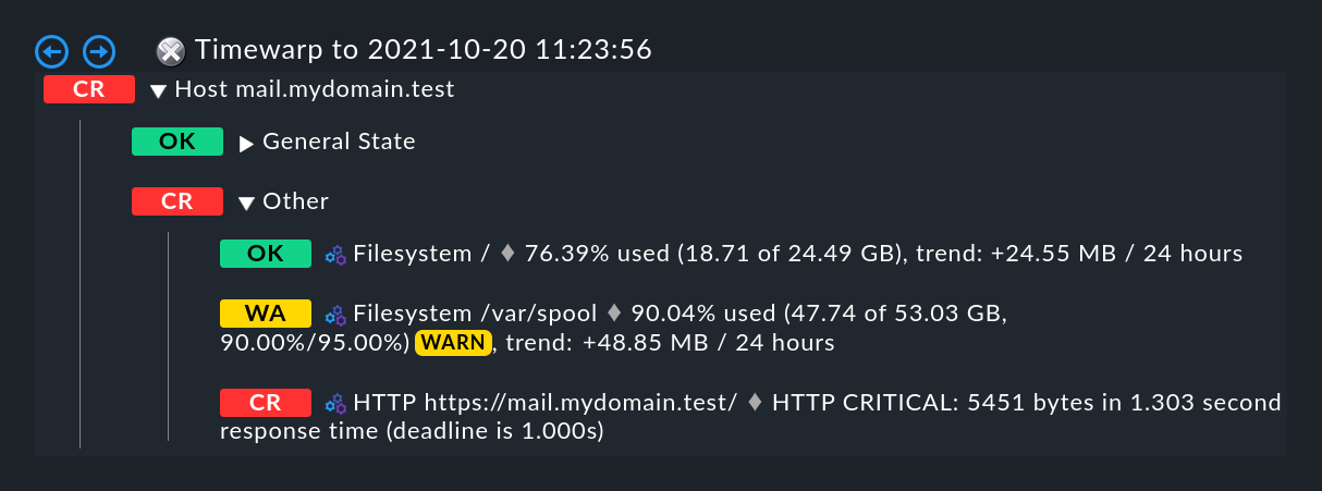
Do you want to know what the cause of the outage was? A simple click
![]() on the magic wand is enough. This enables a journey
through time to the exact point of time when the outage occurred,
and opens a display of the BI aggregation at that time — in the following image,
already opened at the correct location:
on the magic wand is enough. This enables a journey
through time to the exact point of time when the outage occurred,
and opens a display of the BI aggregation at that time — in the following image,
already opened at the correct location:
5. Availability in reports
Availability views can be embedded in reports. The simplest way is via the Add to menu in the menu bar:
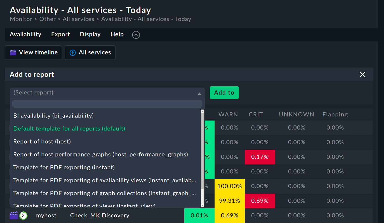
The Availability table report element inserts an availability analysis into the report. All of the options discussed above can be found as parameters directly in the element — although in a slightly different graphic form:
The final option is a special one:

Here you can specify which display should be added to the report:
The availability table
The graphic display of the timeline
The timeline in detail with the individual time periods
Unlike the normal interactive views, here you can simultaneously embed tables and timelines into reports.
A second feature is the specification of the evaluation time period. This option is missing here, because it is predetermined automatically by the report.
The object selection, as with every report element, is either adopted from the report or predefined directly in the element.
6. Technical background
6.1. How the calculations function
For calculating the availability, Checkmk accesses the archived monitoring history logs, and to do so orients itself to the state changes. If, for example, at 5:14 p.m. on 10/20/2021 a service changes its state to CRIT, and then at at 5:24 p.m. changes back to OK, then you know that during this 10 minute time period the service was in a CRIT state.
These state changes are recorded in the Monitoring log, have the alert type
HOST ALERT or SERVICE ALERT, and look like this for example:
[1634742874] SERVICE ALERT: mail.mydomain.com;Filesystem /var/spool;CRITICAL;HARD;1;CRIT - 95.9% used (206.96 of 215.81 GB), (warn/crit at 90.00/95.00%), trend: 0.00 B / 24 hoursThere is always a current log file which includes entries for the most recent activity up to the present point in time, as well as a directory with an archive of the preceding periods. The location of these files varies, depending on the monitoring core in use:
| Core | Current file | Older files |
|---|---|---|
|
|
|
|
|
The user interface does not access these files directly, rather it queries them using a Livestatus-query issued from the monitoring core. Among other factors, this is important since in a distributed monitoring the history files are not stored on the same system as the GUI.
The Livestatus query makes use of the statehist table. In contrast to
the log table – which provides a ‘naked’ access to the history — here the statehist table is used because it has already performed the
initial time-consuming calculation steps. Among other things it assumes the task
of checking back in the history to determine the initial state, and the
calculation of time periods with the same state, with their starts,
durations and ends.
The condensing of the states procedure is performed in the user overview by the Availability Module, as described at the beginning of this article.
6.2. The availability cache in CMC
How the cache works
![]() For queries that reach far back into the past, many log
files must be processed accordingly. That obviously has a negative effect on
the duration of the calculation. For this reason, in the Checkmk
Micro Core there is a very efficient cache of the monitoring history,
in which from the start all important information on objects' changes of state
has already been determined from the log files held in RAM, and which is
continuously updated in the active monitoring.
The consequence of this is that all availability queries can be
answered directly and very efficiently from the RAM, and thus no further
access is required.
For queries that reach far back into the past, many log
files must be processed accordingly. That obviously has a negative effect on
the duration of the calculation. For this reason, in the Checkmk
Micro Core there is a very efficient cache of the monitoring history,
in which from the start all important information on objects' changes of state
has already been determined from the log files held in RAM, and which is
continuously updated in the active monitoring.
The consequence of this is that all availability queries can be
answered directly and very efficiently from the RAM, and thus no further
access is required.
Parsing the log files is very rapid, and with suitably fast hard drives can achieve a processing speed of up to 80 MB/sec! So that creating the cache does not delay the start of the monitoring, this is performed asynchronously — from the present back to the past in fact. A short delay will be noticeable if directly following the start of the Checkmk site an availability query covering a long time range is initiated immediately. In such a situation it is possible that the cache does not yet reach far enough back into the past, and that the GUI needs a few moments to think about it.
With an Activate changes the cache is retained! Only with an actual (re)start of Checkmk will it need to be newly generated — for example, following a server reboot or an update of Checkmk.
Cache statistics
If you are curious about how long the generation of a cache could take,
a statistic can be found in the var/log/cmc.log log file. Here is an
example from a smaller monitoring system:
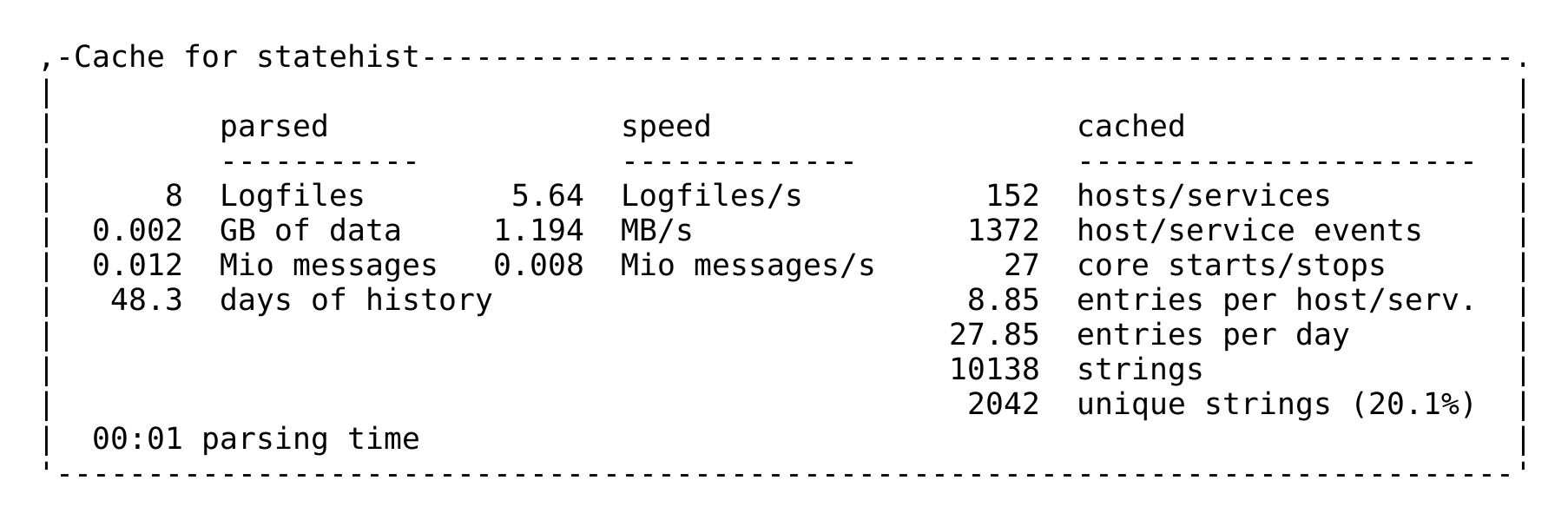
Tuning the cache
In order to keep the cache’s storage requirement under control, it is limited to a horizon of up to 730 days into the past. This limit is fixed — thus queries reaching further back into the past are not merely slower, they are impossible. This can be easily customized using the Global Settings > Monitoring Core > In-memory cache for availability data global setting:
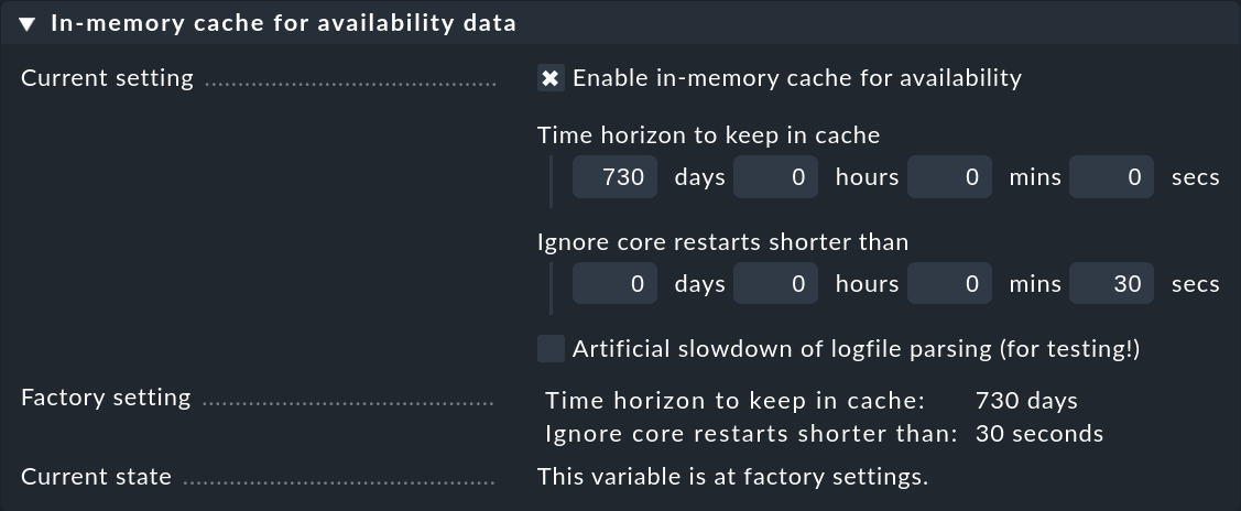
Alongside the horizon for the calculation, additionally there is a second interesting setting: Ignore core restarts shorter than…. A new start of the core (e.g., for the purpose of an update or server restart) actually produces time periods counting as unmonitored. Outages of up to 30 seconds will thereby simply be ignored. This time can be increased and longer times can also be simply suppressed. The availability calculation will then assume that all hosts and services have maintained their respective last communicated states for the whole time.
7. Files and directories
| File path | Function |
|---|---|
|
Current log file for the monitoring history in the CMC |
|
Directory with the history’s older log files |
|
The CMC’s log file, in which the availability cache’s statistics can be viewed |
|
The current log file for Nagios’ monitoring history |
|
Directory with the older log files in Nagios |
|
Here the annotations and retrospectively-amended scheduled downtimes for outages are stored. The file is in the Python-format and can be manually edited. |